Expected Default Frequency Explained With Easy Examples

TL;DR

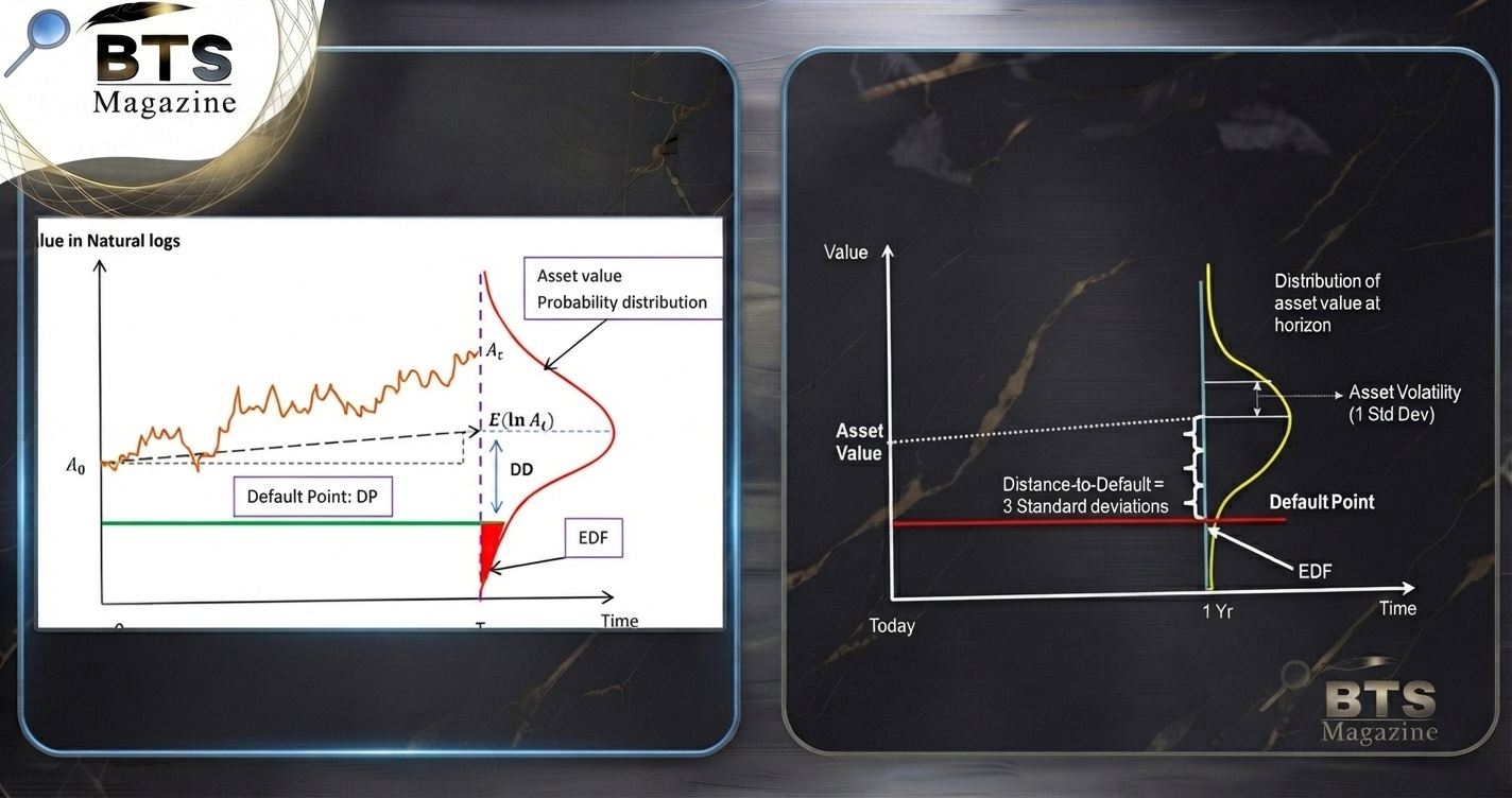
Expected Default Frequency (EDF) is a credit-risk measure that estimates the probability that a company will default on its financial obligations within a specified period, commonly one year. It is strongly associated with structural credit-risk models such as the Moody’s KMV approach.

A higher EDF generally means greater estimated default risk, while a lower EDF suggests stronger credit quality. EDF models typically consider a company’s asset value, debt obligations, market information, asset volatility, and its distance to default.

Featured Snippet: What Is Expected Default Frequency?

Expected Default Frequency (EDF) is an estimate of the probability that a company will default on its debt within a given period. In common public-firm applications, the horizon is one year. EDF models analyze how far a company’s estimated asset value is from a level at which its financial obligations may become unsustainable.

Put simply, EDF attempts to answer:

“How likely is this borrower to default during the period being measured?”

An EDF of 1%, for example, represents an estimated 1% probability of default over the applicable horizon. It does not mean that the company will definitely default.

What Is Expected Default Frequency?

Expected Default Frequency is a quantitative measure used in credit-risk analysis.

It is particularly associated with the KMV framework and Moody’s credit-risk analytics. Moody’s describes its Public Firm EDF measure as an estimated probability of default and notes that the structural framework evolved from the work of Black, Scholes, and Merton.

Unlike a traditional credit score that simply places a borrower into a broad category, EDF attempts to produce a numerical estimate.

For example:

• EDF = 0.05%: very low modeled default probability
• EDF = 0.50%: higher, but still relatively modest, modeled risk
• EDF = 3.00%: substantially greater default risk
• EDF = 10.00%: very high modeled default risk

These percentages should never be interpreted in isolation. The company’s industry, economic environment, debt maturity structure, model methodology, and time horizon also matter.

Why Is Expected Default Frequency Important?

Lenders and investors face a simple problem whenever they provide capital:

Will the borrower repay them?

EDF helps turn that question into a measurable risk estimate.

Financial institutions can use probability-of-default measures when assessing borrowers, managing credit portfolios, pricing debt, setting exposure limits, and monitoring changes in credit quality.

Probability of default is also an important concept in banking regulation. Under the Basel framework’s Internal Ratings-Based approach, a one-year probability of default is an important risk component for corporate, sovereign, and bank exposures.

EDF can therefore help analysts move beyond statements such as:

“This company looks risky.”

Instead, they can think in terms such as:

“The modeled probability of default has increased materially during the last six months.”

That distinction makes credit analysis more systematic.

How Does Expected Default Frequency Work?

The basic logic behind EDF is easier to understand than the mathematics might suggest.

Imagine a company has assets worth significantly more than the level of debt that could push it into financial distress.

There is a large financial cushion.

Now imagine another company whose asset value is only slightly above its critical debt level.

Even a relatively small decline in asset value could place that company in serious difficulty.

EDF models attempt to quantify this risk by examining the relationship among:

1. Company asset value
2. Asset volatility
3. Debt obligations
4. Default threshold or default point
5. Time horizon
6. Distance to default
7. Observed historical default experience

The closer the company moves toward its default threshold—and the more volatile its assets become—the greater its estimated default risk will generally be.

Moody’s describes the Public Firm EDF framework as a structural credit-risk model and uses EDF as an estimated probability of default in applications such as bond valuation.

What Is the Merton Model’s Connection to EDF?

To understand EDF properly, it helps to understand the Merton model.

Robert C. Merton’s influential 1974 work modeled corporate debt and default risk by linking a company’s obligations to the value of its underlying assets. His research became foundational to structural credit-risk modeling.

The basic economic idea is straightforward.

Think of a company as having:

Assets = Debt + Equity

If the company’s asset value remains comfortably above its debt obligations, shareholders retain economic value.

If asset values fall far enough, however, the company may no longer be able to satisfy its obligations.

The KMV approach developed this structural idea into a practical credit-risk framework. The model is commonly associated with estimating a firm’s distance to default and then translating that measure into a probability of default, or EDF.

What Is Distance to Default?

Distance to Default (DD) measures how far a company’s estimated asset value is from its default threshold, typically expressed relative to asset volatility.

In simple language:

Distance to default measures the size of a company’s financial safety cushion after accounting for uncertainty in its asset value.

A company with a large distance to default is generally considered less likely to cross the default threshold.

A company with a small distance to default has less room for financial deterioration.

A simplified conceptual formula is:

Distance to Default ≈ Financial Cushion ÷ Asset Risk

Suppose:

• Estimated company asset value = $500 million
• Estimated default point = $300 million
• Financial cushion = $200 million

If the company’s assets are relatively stable, that $200 million cushion may represent substantial protection.

However, if the company’s asset value fluctuates dramatically, the same $200 million cushion may provide considerably less protection.

This is why volatility matters as much as leverage in structural credit analysis.

How Is Expected Default Frequency Calculated?

The exact methodologies used in commercial EDF systems can be sophisticated and proprietary, but the conceptual process can be understood in several stages.

1. Estimate the market value of the company’s assets

For publicly traded companies, analysts can observe equity market capitalization directly.

The total market value of company assets is not normally observable in the same way.

Structural models therefore estimate asset value using equity value, debt information, and market-based relationships.

2. Estimate asset volatility

A company whose underlying asset value changes rapidly is more likely to experience a sufficiently large decline to reach its default point.

Higher volatility therefore generally increases default risk, all else equal.

3. Determine the default point

The model identifies a level of liabilities at which financial distress or default becomes economically plausible.

Traditional explanations of KMV often relate this default point to short-term liabilities plus a portion of longer-term debt rather than simply treating every dollar of debt as immediately payable.

4. Calculate distance to default

The difference between expected asset value and the default point is evaluated relative to expected asset volatility.

5. Convert distance to default into EDF

The distance-to-default measure is then mapped into an estimated probability of default.

Commercial implementations may use extensive historical default data and additional model adjustments rather than relying solely on a simple theoretical normal-distribution calculation.

The result is the Expected Default Frequency.

Easy Expected Default Frequency Example

Consider two simplified companies.

Factor	Company Alpha	Company Beta
Estimated asset value	$800 million	$800 million
Default point	$300 million	$650 million
Financial cushion	$500 million	$150 million
Asset volatility	Low	High
Distance to default	Relatively large	Relatively small
Expected EDF	Lower	Higher

Company Alpha has a substantial cushion between its assets and default point.

Its assets are also relatively stable.

Company Beta has the same total asset value, but much more debt and significantly greater asset volatility.

Beta therefore has a much higher chance of seeing its asset value fall below the critical level.

A structural credit-risk model would generally assign Company Beta the higher EDF.

The lesson is important:

Default risk depends not only on how much debt a company has, but also on the value and volatility of its assets.

Example of Interpreting an EDF Percentage

Assume an analytical model gives Company XYZ a one-year EDF of 2%.

The correct interpretation is approximately:

Based on the model and available information, the estimated probability of Company XYZ defaulting during the next year is 2%.

It does not mean:

• XYZ will lose 2% of its value.
• Investors will lose exactly 2%.
• Two of every 100 identical companies must default.
• XYZ has a 98% guaranteed chance of survival.
• Its bonds should automatically yield 2% more than Treasury securities.

EDF is a probability estimate, not a guaranteed outcome.

Real-world default outcomes can differ from model predictions.

What Causes Expected Default Frequency to Increase?

Several developments can push a company’s EDF higher.

Falling share prices

For a public company, a sharp decline in equity value may signal a reduction in the market value of the firm’s assets or worsening expectations.

Increasing volatility

A volatile company has a greater chance of experiencing a large enough decline to approach the default threshold.

More debt

Additional borrowing can reduce the cushion between asset value and the company’s effective default point.

Weak financial performance

Falling revenue, shrinking margins, negative cash flow, or persistent losses can weaken credit quality.

Economic stress

Recessions, credit-market tightening, commodity shocks, geopolitical disruptions, and industry-specific downturns can all increase default risk.

A real-world illustration can be seen in Moody’s analysis of Boeing: its EDF rose substantially during the period surrounding the 737 MAX crisis and the COVID-19 disruption, illustrating how business stress and broader economic shocks can affect modeled default probabilities.

What Can Cause EDF to Fall?

EDF can decline when a company’s financial position strengthens.

Possible drivers include:

• Rising market value
• Lower share-price volatility
• Reduced debt
• Improved cash flow
• Stronger profitability
• Longer debt maturities
• Successful refinancing
• Improved industry conditions
• Greater access to liquidity

Suppose a business uses excess cash to repay $400 million of debt while operating performance improves.

Its financial cushion increases.

If asset volatility also declines, its distance to default may rise substantially.

The resulting EDF may therefore fall.

EDF vs. Probability of Default

EDF and Probability of Default (PD) are closely related concepts.

In practical terms, EDF is a modeled probability-of-default measure associated with particular credit-risk methodologies.

PD is the broader generic term.

Feature	EDF	Probability of Default
Meaning	Estimated likelihood of default	Estimated likelihood of default
Scope	Often associated with specific credit models	General credit-risk concept
Typical horizon	Commonly one year, though term structures can exist	Depends on model
Inputs	May include market, debt, volatility and financial data	Depends on methodology
Use	Credit monitoring, portfolio analysis, pricing	Banking, lending, regulation, investing

The important point is that EDF is a type of default-probability measure, but not every PD model is an EDF model.

EDF vs. Credit Rating

EDF should also not be confused with a credit rating.

A credit rating typically places an issuer or security into an ordinal category such as:

• AAA
• AA
• A
• BBB
• BB
• B

EDF produces a numerical probability estimate.

A company might therefore experience a meaningful increase in EDF before a traditional rating category changes.

This can make market-sensitive default measures useful as an additional early-warning indicator.

However, the two measures answer somewhat different questions and may use different methodologies. EDF should complement rather than automatically replace broader credit analysis.

EDF vs. Expected Loss

Another common mistake is treating probability of default and expected credit loss as the same thing.

They are not.

Expected loss depends on more than the likelihood of default.

A simplified credit-risk relationship is:

Expected Loss = PD × LGD × EAD

Where:

• PD = Probability of Default
• LGD = Loss Given Default
• EAD = Exposure at Default

The Basel framework also uses probability of default and loss given default as important components of credit-risk calculations.

Consider two $1 million loans with the same 2% default probability.

If one loan is secured by highly valuable collateral and the other is unsecured, their expected losses can differ considerably even though their PDs are identical.

EDF therefore tells you about default likelihood, not necessarily the size of the eventual loss.

EDF vs. Credit Spread

A credit spread is the additional yield investors demand for holding risky debt relative to an appropriate benchmark.

EDF is an estimate of default probability.

They are connected, but they are not interchangeable.

Bond spreads can reflect:

• Expected default losses
• Recovery expectations
• Liquidity
• Risk premiums
• Market sentiment
• Security seniority
• Maturity
• Supply and demand

Moody’s EDF-based bond valuation research explicitly links EDF with loss given default and other market-wide parameters when estimating bond spreads, illustrating why default probability alone does not determine a bond’s spread.

How Banks and Investors Use EDF

EDF can be useful in several real-world situations.

Credit screening

A lender can compare the modeled default risk of potential borrowers before extending credit.

Portfolio monitoring

Institutions can track whether EDF levels are rising across particular borrowers, sectors, or regions.

Early-warning systems

A sudden increase in EDF may trigger additional credit review.

Bond analysis

Investors can compare market spreads with modeled credit risk to evaluate whether securities appear relatively expensive or cheap.

Risk limits

Financial institutions may use default-probability measures when setting exposure limits for counterparties.

Stress testing

Analysts can examine how weaker asset values, greater volatility, or higher leverage might affect default risk under adverse scenarios.

These applications are especially valuable when EDF is used alongside fundamental financial analysis rather than treated as a stand-alone decision rule.

Advantages of Expected Default Frequency

EDF has several important strengths.

It produces a quantitative result. Analysts receive a probability estimate rather than only a broad qualitative description.

It can be market sensitive. Public-firm models can incorporate changing equity-market information.

It accounts for leverage and volatility. Two companies with similar debt levels can have very different risk profiles.

It supports comparison. Analysts can track the same borrower through time or compare multiple firms using a consistent framework.

It can provide early-warning information. Market-based indicators can sometimes deteriorate quickly when investors reassess a company’s prospects.

These characteristics explain why structural probability-of-default models remain important tools in modern credit analysis.

Limitations of Expected Default Frequency

No credit model should be treated as infallible.

EDF has limitations that analysts must understand.

Asset value must be estimated

For public companies, equity is observable, but the total market value of corporate assets usually is not.

Models therefore rely on estimation.

Market volatility can create noise

Stock markets can move sharply because of temporary sentiment rather than permanent deterioration in credit quality.

Model assumptions matter

Structural models simplify complex corporate financing structures and may not perfectly capture liquidity crises, covenant breaches, government intervention, fraud, or abrupt operational shocks.

Private companies are harder to assess

Private firms lack continuously traded equity prices, so models for private companies generally rely more heavily on financial statements and other information.

Moody’s, for example, distinguishes between public-firm EDF approaches and RiskCalc models that use company financial information to estimate default risk.

EDF is not certainty

A company with a very low estimated EDF can still default.

A company with a high EDF may recover.

Probability models describe risk—not destiny.

How to Read EDF Like a Credit Analyst

A good analyst rarely asks only:

“What is the EDF today?”

A better analysis asks:

• Is EDF rising or falling?
• How quickly has it changed?
• What caused the movement?
• Has leverage increased?
• Has equity value fallen?
• Has volatility increased?
• Is liquidity deteriorating?
• Are major debt maturities approaching?
• Is the entire sector weakening?
• Does fundamental analysis confirm the signal?

For example, an increase from 0.20% to 0.40% may still represent relatively low absolute risk, but the doubling itself deserves investigation.

Likewise, a decline from 12% to 8% represents improvement, yet the company may remain financially vulnerable.

Direction, magnitude, context, and absolute level all matter.

Frequently Asked Questions About Expected Default Frequency

What does EDF mean in finance?

EDF means Expected Default Frequency. It is a credit-risk measure used to estimate the probability that a borrower or company will default during a specified period.

Is a high EDF good or bad?

A high EDF generally indicates higher estimated default risk, while a low EDF indicates lower modeled default risk.

What does a 1% EDF mean?

A one-year EDF of 1% means the model estimates approximately a 1% probability of default during the next year, subject to the methodology and information used.

Is EDF the same as a credit score?

No. EDF is a probability-based credit-risk measure. A credit score or rating normally places borrowers into categories or scoring bands.

What is distance to default?

Distance to default measures how far a company’s estimated asset value is from its default threshold after considering asset volatility.

Does a low EDF guarantee that a company will not default?

No. EDF is a statistical estimate. Unexpected events can cause even apparently strong companies to experience financial distress.

Can EDF change quickly?

Yes. Market-sensitive EDF measures may respond to changes in stock prices, volatility, leverage, and broader economic conditions.

Final Thoughts

Expected Default Frequency provides a practical way to translate corporate financial strength, leverage, asset volatility, and market information into an estimated probability of default.

The most useful way to interpret EDF is not as a crystal ball, but as a risk signal.

A low EDF suggests that a company currently appears relatively far from financial distress. A rising EDF tells analysts that risk may be building. A high EDF signals that closer investigation is warranted.

Professional credit analysis therefore combines EDF with financial statements, cash-flow forecasts, debt maturity schedules, liquidity analysis, industry conditions, collateral values, and qualitative judgment.

For readers who want to explore the broader theory behind EDF, the concept is closely connected with Robert C. Merton’s structural approach to corporate credit risk. His landmark 1974 research established a foundation for modeling default through the relationship between corporate assets and liabilities, while later KMV-style models developed practical approaches for translating distance to default into Expected Default Frequency. For additional background, Wikipedia’s article on Probability of Default provides a useful introduction to the broader default-probability concept and its role in modern credit-risk analysis.

Internal Linking Suggestions

Use contextual internal links to related content such as:

• Probability of Default Explained
• Credit Risk Explained
• Loss Given Default (LGD)
• Exposure at Default (EAD)
• Expected Credit Loss
• Merton Model Explained
• Credit Ratings Explained
• Debt-to-Equity Ratio
• How to Analyze Corporate Bonds

External Authority Link Suggestions

For stronger EEAT signals, consider referencing:

• Moody’s research explaining EDF credit measures and EDF-based bond valuation.
• Bank for International Settlements / Basel Committee guidance covering probability of default in bank credit-risk frameworks.
• Robert C. Merton’s 1974 Journal of Finance paper, On the Pricing of Corporate Debt: The Risk Structure of Interest Rates.